This post is an excerpt from the video series 4 Essential Microsoft Excel Skills Every Marketer Should Learn. If you want to become a master of the almighty spreadsheet, watch the full video series here.
I know, I know … “VLOOKUP function” sounds like the geekiest, most complicated thing ever.
But trust me: as was the case with pivot tables, Microsoft Excel's VLOOKUP function is easier to use than you think. What’s more, it is incredibly powerful, and is definitely something you want to have in your arsenal of analytical weapons.
So, what does VLOOKUP do, exactly? Here’s the simple explanation: The VLOOKUP function searches for a specific value in your data, and once it identifies that value, it can find -- and display -- some other piece of information that’s associated with that value.
VLOOKUP Example
You could use the VLOOKUP formula to transfer revenue data from a separate spreadsheet and match it with the appropriate customer based on a common identifier like customer ID or email address. In this example, VLOOKUP enables you to easily see revenue by customer without searching, copying, and pasting for each individual cell.
In practical terms, this means you can take the revenue data from your second spreadsheet and integrate it with the customer data in your first spreadsheet in order to reveal the bigger picture about your business's performance.
Below, you'll see a five-step guide to performing this VLOOKUP example, followed by a video tutorial for using VLOOKUP to organize a list of blog posts.
How Does VLOOKUP Work?
The secret to how VLOOKUP works? Unique identifiers.
A unique identifier is a piece of information that both of your data sources share, and -- as its name implies -- it is unique (i.e. the identifier is only associated with one record in your database). Unique identifiers include product codes, stock keeping units (SKUs), and customer contacts.
Since HubSpot and most CRMs both use email addresses to uniquely identify the contacts in their databases, HubSpot customers can use “email address” as their unique identifier to execute a VLOOKUP.
Steps to Using VLOOKUP in Excel
Take the VLOOKUP example above. Let’s say you’re looking through your HubSpot data and are checking out which of your site pages your contacts have viewed. You’re also paying attention to whether or not any of those contacts have converted into customers.
Then it hits you: In addition to knowing which of those contacts have closed, you want to know how much MRR (monthly recurring revenue) each of them brings in. That way, you can tie your revenue back to your site pages and do some analysis to see which pages are having the biggest impact on your bottom line.
There’s only one problem: Your MRR data lives in your CRM. And while you could manually look up each and every contact in your CRM to find their MRR, and then manually match those values to their corresponding contacts in your HubSpot data, the whole process would be ridiculously time-consuming and impractical.
That’s where the VLOOKUP function comes in. For your reference, here's what a VLOOKUP function looks like:
VLOOKUP(lookup_value , table_array , col_index_num , range_lookup)
In the steps below, we'll assign the right value to each of these components, using customer names as our unique identifier to find the MRR of each customer.
Step 1: Identify a Column of Cells You'd Like to Fill With New Data
If this data is coming from a pivot table made in Excel, copy the data into a new spreadsheet so the VLOOKUP function can freely read this data.
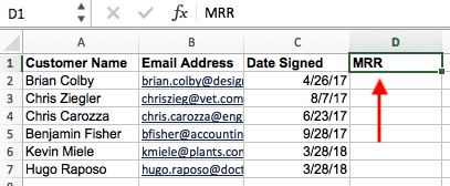
Then, label a column next to the cells you want more information on with a proper title in the top cell, such as "MRR," for monthly recurring revenue. This new column is where the data you're fetching will go.
Step 2: Select 'Function' (Fx) > VLOOKUP and Enter Your Starting Cell
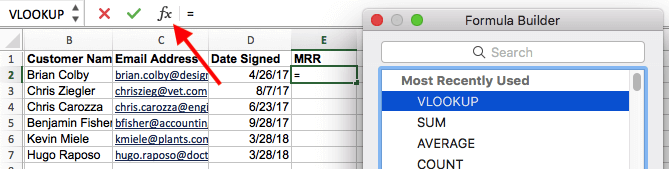
To the left of the text bar above your spreadsheet, you'll see a small function icon that looks like a script "Fx." Click on the first empty cell beneath your column title and then click this function icon.
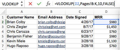
Select "VLOOKUP" from the list of options that appears, and then re-click the cell you've highlighted and enter the cell you're trying to find a match for. In this case, it's A2. You'll start migrating your new data into E2, since this cell represents the MRR of the customer name listed in A2.
Step 3: Enter the Table Array and Column Number You're Searching Through
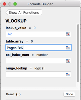
Then, next to the "table array" field, enter the range of cells you'd like to search and the sheet where these cells are located. The VLOOKUP form will help you fetch the correct page.
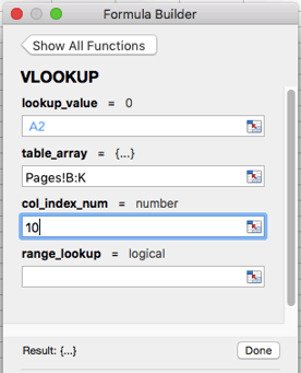
Beneath this field, you'll also enter the "column index number" of the table array you're searching through. For example, if you're focusing on columns B through K (notated "B:K" when entered in the "table array" field), but the specific values you want are in column K, you'll enter "10" in the "column index number" field, since column K is the 10th column from the left.
Step 4: Enter Your Range Lookup
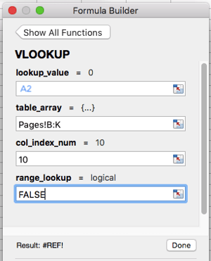
In contexts like monthly revenue, you want to find exact matches from the table you're searching through. To do this, enter 'FALSE' in the "range lookup" field. This tells Excel you want to find only the exact revenue associated with each sales contact.
Step 5: Click 'Done' (or 'Enter') and Fill Your New Column
In order to officially bring in the values you want into your new column from Step 1, click "Done" (or "Enter," depending on your version of Excel) after filling the "range lookup" field. This will populate your first cell. You might take this opportunity to look in the other spreadsheet to make sure this was the correct value.
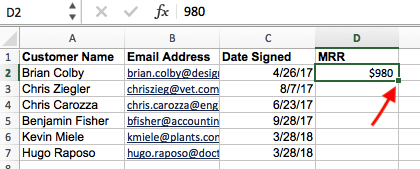
If so, populate the rest of the new column with each subsequent value by clicking the first filled cell, then clicking the tiny square that appears on the bottom-right corner of this cell. Done! All your values should appear.
Alright, enough explanation: let's see another example of the VLOOKUP in action!
In the video below, we're taking the pivot table we made in video #2, pasting the values into a new sheet, and using it as an example report. We then use the VLOOKUP function to match blog post authors (from our second data source) to their corresponding post titles. In this instance, we're using post title as our unique identifier.
Author's note: Keep in mind there are many different versions of Excel, so what you see in the video above might not always match up exactly with what you'll see in your version. That's why we encourage you to download the written instructions and demo data so you can follow along.
Download demo data | Download instructions (Mac) | Download instructions (PC)
Want to learn to do more in Excel? Download the full video series, 4 Essential Microsoft Excel Skills Every Marketer Should Learn.

No comments:
Post a Comment